
Streaming Machine learning pipeline for Sentiment Analysis using Apache APIs: Kafka, Spark and Drill - Part 1
October 28, 2020Editor’s Note: MapR products and solutions sold prior to the acquisition of such assets by Hewlett Packard Enterprise Company in 2019, may have older product names and model numbers that differ from current solutions. For information about current offerings, which are now part of HPE Ezmeral Data Fabric, please visit https://www.hpe.com/us/en/software/data-fabric.html
Original Post Information:
"authorDisplayName": ["Carol McDonald"],
"publish": "2019-05-07T07:00:00.000Z",
"tags": "machine-learning"
Text mining and analysis of social media, emails, support tickets, chats, product reviews, and recommendations have become a valuable resource used in almost all industry verticals to study data patterns in order to help businesses to gain insights, understand customers, predict and enhance the customer experience, tailor marketing campaigns, and aid in decision-making.
Sentiment analysis uses machine learning algorithms to determine how positive or negative text content is. Example use cases of sentiment analysis include:
- Quickly understanding the tone from customer reviews
- To gain insights about what customers like or dislike about a product or service
- To gain insights about what might influence buying decisions of new customers
- To give businesses market awareness
- To address issues early
- Understanding stock market sentiment to gain insights for financial signal predictions
- Determining what people think about customer support
- Social media monitoring
- Brand/product/company popularity/reputation/perception monitoring
- Discontented customer detection monitoring and alerts
- Marketing campaign monitoring/analysis
- Customer service opinion monitoring/analysis
- Brand sentiment attitude analysis
- Customer feedback analytics
- Competition sentiment analytics
- Brand influencers monitoring
Manually analyzing the abundance of text produced by customers or potential customers is time-consuming; machine learning is more efficient and with streaming analysis, insights can be provided in real time.
This is the first in a series of blog posts, which discusses the architecture of a data pipeline that combines streaming data with machine learning and fast storage. In this first part, we will explore sentiment analysis using Spark machine learning data pipelines. We will work with a dataset of Amazon product reviews and build a machine learning model to classify reviews as positive or negative. In the second part of this tutorial, we will use this machine learning model with streaming data to classify documents in real time. The second post will discuss using the saved model with streaming data to do real-time analysis of product sentiment, storing the results in MapR Database, and making them rapidly available for Spark and Drill SQL.

In this post, we will go over the following:
- Overview of classification and sentiment analysis concepts
- Building feature vectors from text documents
- Training a machine learning model to classify positive and negative reviews using logistic regression
- Evaluating and saving the machine learning model
Classification
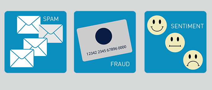
Classification is a family of supervised machine learning algorithms that identify which category an item belongs to (such as whether an email is spam or not), based on labeled data (such as the email subject and message text). Some common use cases for classification include credit card fraud detection, email spam detection, and sentiment analysis.
Classification takes a set of data with known labels and predetermined features and learns how to label new records, based on that information. Features are the properties that you can use to make predictions. To build a classifier model, you explore and extract the features that most contribute to the classification.

Let's go through an example for sentiment analysis for text classification of positive or negative.
- What are we trying to predict?
- In this example, the customer review ratings are used to label reviews as positive or not. A review with 4 to 5 stars is considered a positive review, and a review with 1 to 2 stars is considered a negative review.
- What are the properties that you can use to make predictions?
- The review text words are used as the features to discover positive or negative similarities in order to categorize customer text sentiment as positive or negative.
Machine Learning Workflow
Using Machine Learning is an iterative process, which involves:
- Data discovery and model creation
- Analysis of historical data
- Identifying new data sources, which traditional analytics or databases are not using, due to the format, size, or structure
- Collecting, correlating, and analyzing data across multiple data sources
- Knowing and applying the right kind of machine learning algorithms to get value out of the data
- Training, testing, and evaluating the results of machine learning algorithms to build a model
- Using the model in production to make predictions
- Data discovery and updating the model with new data

Feature Extraction
Features are the interesting properties in the data that you can use to make predictions. Feature engineering is the process of transforming raw data into inputs for a machine learning algorithm. In order to be used in Spark machine learning algorithms, features have to be put into feature vectors, which are vectors of numbers representing the value for each feature. To build a classifier model, you extract and test to find the features of interest that most contribute to the classification.

Apache Spark for Text Feature Extraction
The TF-IDF (Term Frequency–Inverse Document Frequency) feature extractors in SparkMLlib can be used to convert text words into feature vectors. TF-IDF calculates the most important words in a single document compared to a collection of documents. For each word in a collection of documents, it computes:
- Term Frequency (TF), which is the number of times a word occurs in a specific document
- Document Frequency (DF), which is the number of times a word occurs in a collection of documents
- Term Frequency-Inverse Document Frequency (TF-IDF), which measures the significance of a word in a document (the word occurs a lot in that document, but is rare in the collection of documents)
For example, if you had a collection of reviews about bike accessories, then the word 'returned' in a review would be more significant for that document than the word 'bike.'In the simple example below, there is one positive text document and one negative text document, with the word tokens 'love,''bike,' and 'returned' (after filtering to remove insignificant words like 'this' and 'I'). The TF, DF, and TF-IDF calculations are shown. The word 'bike' has a TF of 1 in 2 documents (word count in each document), a document frequency of 2 (word count in set of documents), and a TF-IDF of ½ (TF divided by DF).

Logistic Regression
Logistic regression is a popular method to predict a binary response. It is a special case of generalized linear models that predicts the probability of the outcome. Logistic regression measures the relationship between the Y "Label" and the X "Features" by estimating probabilities using a logistic function. The model predicts a probability, which is used to predict the label class.

In our text classification case, logistic regression tries to predict the probability of a review text being positive or negative, given the label and feature vector of TF-IDF values. Logistic regression finds the best fit weight for each word in the collection of text by multiplying each TF-IDF feature by a weight and passing the sum through a sigmoid function, which transforms the input x into the output y, a number between 0 and 1. In other words, logistic regression can be understood as finding the parameters that best fit:


Logistic regression has the following advantages:
- Can handle sparse data
- Fast to train
- Weights can be interpreted
- Positive weights will correspond to the words that are positive
- Negative weights will correspond to the words that are negative
Data Exploration and Feature Extraction
We will be using a dataset of Amazon sports and outdoor products review data, which you can download here: http://jmcauley.ucsd.edu/data/amazon/. The dataset has the following schema:
*Italicized fields are for sentiment analysis
reviewerID - ID of the reviewer, e.g., A2SUAM1J3GNN3Basin - ID of the product, e.g., 0000013714reviewerName - name of the reviewerhelpful - helpfulness rating of the review, e.g., 2/3
*reviewText - text of the review
*overall - rating of the product
*summary - summary of the reviewunixReviewTime - time of the review (Unix time)reviewTime - time of the review (raw)
The dataset has the following JSON format:
{
    "reviewerID": "A1PUWI9RTQV19S",
    "asin": "B003Y5C132",
    "reviewerName": "kris",
    "helpful": [0, 1],
    "reviewText": "A little small in hind sight, but I did order a .30 cal box. Good condition, and keeps my ammo organized.",
    "overall": 5.0,
    "summary": "Nice ammo can",
    "unixReviewTime": 1384905600,
    "reviewTime": "11 20, 2013"
}
In this scenario, we will use logistic regression to predict the label of positive or not, based on the following:
Label :
- overall - rating of the product 4-5 = 1 Positive
- overall - rating of the product 1-2 = 0 Negative
Features :
- reviewText + summary of the review → TF-IDF features
USING THE SPARK ML PACKAGE
Spark ML provides a uniform set of high-level APIs, built on top of DataFrames with the goal of making machine learning scalable and easy. Having ML APIs built on top of DataFrames provides the scalability of partitioned data processing with the ease of SQL for data manipulation.

We will use an ML Pipeline to pass the data through transformers in order to extract the features and an estimator to produce the model.
- Transformer: A transformer is an algorithm that transforms one
DataFrameinto anotherDataFrame. We will use transformers to get aDataFramewith a features vector column. - Estimator: An estimator is an algorithm that can be fit on a
DataFrameto produce a transformer. We will use a an estimator to train a model, which can transform input data to get predictions. - Pipeline: A pipeline chains multiple transformers and estimators together to specify an ML workflow.
Load the Data from a File into a DataFrame
The first step is to load our data into a DataFrame. Below, we specify the data source format and path to load into a DataFrame. Next, we use the withColumn method to add a column combining the review summary with the review text, and we drop columns that are not needed.
import org.apache.spark._
import org.apache.spark.ml._
import org.apache.spark.sql._

var file ="/user/mapr/data/revsporttrain.json"

val df0  = spark.read.format("json")
 .option("inferSchema", "true")
 .load(file)

val df = df0.withColumn("reviewTS",
  concat($"summary", lit(" "),$"reviewText"))
 .drop("helpful")
 .drop("reviewerID")
 .drop("reviewerName")
 .drop("reviewTime")
The DataFrame printSchema displays the schema:
df.printSchema

root
 |-- asin: string (nullable = true)
 |-- overall: double (nullable = true)
 |-- reviewText: string (nullable = true)
 |-- summary: string (nullable = true)
 |-- unixReviewTime: long (nullable = true)
 |-- reviewTS: string (nullable = true)
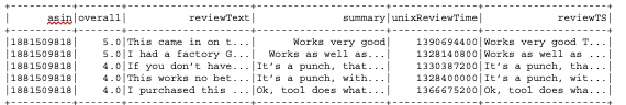
The DataFrame show method displays the first 20 rows or the specified number of rows:
df.show(5)
Summary Statistics
Spark DataFrames include some built-in functions for statistical processing. The describe() function performs summary statistics calculations on all numeric columns and returns them as a DataFrame. Below, we analyze the product rating overall column:
df.describe("overall").show

**result:**
+-------+------------------+
|**summary**|           **overall**|
+-------+------------------+
|  **count**|            **200000**|
|   **mean**|          **4.395105**|
| **stddev**|**0.9894654790262587**|
|    **min**|               **1.0**|
|    **max**|               **5.0**|
+-------+------------------+
In the code below, we filter to remove neutral ratings (=3), then a Spark Bucketizer is used to add a label 0/1 column to the dataset for Positive (overall rating >=4) and not positive (overall rating <4) reviews. Then, the resulting total counts are displayed. Grouping the data by the label column and counting the number of instances in each group shows that there are roughly 13 times as many positive samples as not positive samples.
val df1 = df.filter("overall !=3")

val bucketizer = new Bucketizer()
.setInputCol("overall")
.setOutputCol("label")
.setSplits(Array(Double.NegativeInfinity, 4.0,
 Double.PositiveInfinity))

val df2= bucketizer.transform(df1)

df2.groupBy("overall","label").count.show

**result:**
+-------+-----+------+
|**overall**|**label**| **count**|
+-------+-----+------+
|    **2.0**|  **0.0**|  **6916**|
|    **5.0**|  **1.0**|**127515**|
|    **1.0**|  **0.0**|  **6198**|
|    **4.0**|  **1.0**| **43303**|
+-------+-----+------+
Stratified Sampling
In order to ensure that our model is sensitive to the negative samples, we can put the two sample types on the same footing using stratified sampling. The DataFrames sampleBy() function does this when provided with fractions of each sample type to be returned. Here, we're keeping all instances of negative, but downsampling the negative instances to 10%, then displaying the results.
val fractions = Map(1.0 -> .1, 0.0 -> 1.0)
val df3 = df2.stat.sampleBy("label", fractions, 36L)
df3.groupBy("label").count.show

**result:**

+-----+-----+
|label|count|
+-----+-----+
|  0.0|13114|
|  1.0|17086|
+-----+-----+
Below, the data is split into a training data set and a test data set: 80% of the data is used to train the model, and 20% will be used for testing.
// split into training and test dataset
val splitSeed = 5043
val Array(trainingData, testData) = df3.randomSplit(Array(0.8, 0.2), splitSeed)
Feature Extraction and Pipelining
The ML package needs the label and feature vector to be added as columns to the input DataFrame. We set up a pipeline to pass the data through transformers in order to extract the features and label.
The RegexTokenizer takes an input text column and returns a DataFrame with an additional column of the text split into an array of words by using the provided regex pattern. The StopWordsRemover filters out words which should be excluded, because the words appear frequently and don't carry as much meaning – for example, 'I,' 'is,' 'the.'
In the code below, the RegexTokenizer will split up the column with the review and summary text into a column with an array of words, which will then be filtered by the StopWordsRemover:
val tokenizer = new RegexTokenizer()
.setInputCol("reviewTS")
.setOutputCol("reviewTokensUf")
.setPattern("\\s+|[,.()\"]")

val remover = new StopWordsRemover()
.setStopWords(StopWordsRemover
.loadDefaultStopWords("english"))
.setInputCol("reviewTokensUf")
.setOutputCol("reviewTokens")
An example of the results of the RegexTokenizer and StopWordsRemover, taking as input column reviewTS and adding the reviewTokens column of filtered words, is shown below:

reviewTS | reviewTokens |
| resistance was good but quality wasn't So it worked well for a couple weeks, but during a lunge workout, it snapped on me. I liked it and thought it was a great product until this happened. I noticed small rips on the band. This could have been the issue. | Array(resistance, good, quality, worked, well, couple, weeks, lunge, workout, snapped, liked, thought, great, product, happened, noticed, small, rips, band, issue) |
A CountVectorizer is used to convert the array of word tokens from the previous step to vectors of word token counts. The CountVectorizer is performing the TF part of TF-IDF feature extraction.
val cv = new CountVectorizer()
.setInputCol("reviewTokens")
.setOutputCol("cv")
.setVocabSize(200000)
An example of the results of the CountVectorizer, taking as input column reviewTokens and adding the cv column of vectorized word counts, is shown below. In the cv column: 56004 is the size of the TF word vocabulary; the second array is the position of the word in the word vocabulary ordered by term frequency across the corpus; the third array is the count of the word (TF) in the reviewTokens text.
reviewTokens | cv |
| Array(resistance, good, quality, worked, well, couple, weeks, lunge, workout, snapped, liked, thought, great, product, happened, noticed, small, rips, band, issue) | (56004,[1,2,6,8,13,31,163,168,192,276,487,518,589,643,770,955,1194,1297,4178,19185],[1.0,1.0,1.0,1.0,1.0,1.0,1.0,1.0,1.0,1.0,1.0,1.0,1.0,1.0,1.0,1.0,1.0,1.0,1.0,1.0]) |
Below the cv column created by the CountVectorizer (the TF part of TF-IDF feature extraction) is the input for IDF. IDF takes feature vectors created from the CountVectorizer and down-weights features which appear frequently in a collection of texts (the IDF part of TF-IDF feature extraction). The output features column is the TF-IDF features vector, which the logistic regression function will use.
// list of feature columns
val idf = new IDF()
.setInputCol("cv")
.setOutputCol("features")
An example of the results of the IDF, taking as input column cv and adding the features column of vectorized TF-IDF, is shown below. In the cv column, 56004 is the size of the word vocabulary; the second array is the position of the word in the word vocabulary ordered by term frequency across the corpus; the third array is the TF-IDF of the word in the reviewTokens text.
cv | features |
| (56004,[1,2,6,8,13,31,163,168,192,276,487,518,589,643,770,955,1194,1297,4178,19185],[1.0,1.0,1.0,1.0,1.0,1.0,1.0,1.0,1.0,1.0,1.0,1.0,1.0,1.0,1.0,1.0,1.0,1.0,1.0,1.0]) | (56004,[1,2,6,8,13,31,163,168,192,276,487,518,589,643,770,955,1194,1297,4178,19185],[1.3167453737971118,1.3189162538557524,1.5214341820160893,1.9425118863569042,2.052613811061827,2.3350290362765134,3.188779919701724,3.245760634740672,3.316430208091361,3.620260266951124,4.115700971877636,4.165254786332365,4.655788580192657,4.32745920096672,4.781242886345692,5.001914248514512,5.008106218762434,5.169529657918772,6.793673717742568,8.990898295078788]) |
The final element in our pipeline is an estimator, a logistic regression classifier, which will train on the vector of labels and features and return a (transformer) model.
// create Logistic Regression estimator
// regularizer parameters avoid overfitting

val lr = new LogisticRegression()
.setMaxIter(100)
.setRegParam(0.02)
.setElasticNetParam(0.3)
Below, we put the Tokenizer, CountVectorizer, IDF, and Logistic Regression Classifier in a pipeline. A pipeline chains multiple transformers and estimators together to specify an ML workflow for training and using a model.
val steps =  Array( tokenizer, remover, cv, idf,lr)
val pipeline = new Pipeline().setStages(steps)

TRAIN THE MODEL

Next, we train the logistic regression model with elastic net regularization. The model is trained by making associations between the input features and the labeled output associated with those features. The pipeline.fit method returns a fitted pipeline model.
val model = pipeline.fit(trainingData)

Note: another option for training the model is to tune the parameters, using grid search, and select the best model, using k-fold cross validation with a Spark CrossValidator and a ParamGridBuilder.
Next, we can get the CountVectorizer and LogisticRegression model from the fitted pipeline model, in order to print out the coefficient weights of the words in the text vocabulary (the word feature importance).
// get vocabulary from the CountVectorizer
val vocabulary = model.stages(2)
.asInstanceOf[CountVectorizerModel]
.vocabulary

// get the logistic regression model
val lrModel = model.stages.last
.asInstanceOf[LogisticRegressionModel]

// Get array of coefficient weights
val weights = lrModel.coefficients.toArray

// create array of word and corresponding weight
val word_weight = vocabulary.zip(weights)

// create a dataframe with word and weights columns
val cdf = sc.parallelize(word_weight)
.toDF("word","weights")
Recall that logistic regression generates the coefficient weights of a formula to predict the probability of occurrence of the feature x (in this case, a word) to maximize the probability of the outcome Y, 1 or 0 (in this case, positive or negative text sentiment). The weights can be interpreted:
- Positive weights will correspond to the words that are positive
- Negative weights will correspond to the words that are negative
Below, we sort the weights in descending order to show the most positive words. The results show that 'great,' perfect,' 'easy,' 'works,' and 'excellent' are the most important positive words.
// show the most positive weighted words
cdf.orderBy(desc("weights")).show(10)

**result:**
+---------+-------------------+
|     **word**|             **weight**|
+---------+-------------------+
|    **great**| **0.6078697902359276**|
|  **perfect**|**0.34404726951273945**|
|**excellent**|**0.28217372351853814**|
|     **easy**|**0.26293906850341764**|
|     **love**|**0.23518819188672227**|
|    **works**|  **0.229342771859023**|
|     **good**| **0.2116386469012886**|
|   **highly**| **0.2044040462730194**|
|     **nice**|**0.20088266981583622**|
|     **best**|**0.18194893152633945**|
+---------+-------------------+
Below, we sort the weights in ascending order to show the most negative words.The results show that 'returned,' 'poor,' 'waste,' and 'useless' are the most important negative words.
// show the most negative sentiment words
cdf.orderBy("weights").show(10)

**result:**
+-------------+--------------------+
|         **word**|              **weight**|
+-------------+--------------------+
|     **returned**|**-0.38185206877117467**|
|         **poor**|**-0.35366409294425644**|
|        **waste**| **-0.3159724826017525**|
|      **useless**| **-0.2914292653060789**|
|       **return**| **-0.2724012497362986**|
|**disappointing**| **-0.2666580559444479**|
|        **broke**| **-0.2656765359468423**|
| **disappointed**|**-0.23852780960293438**|
|    **returning**|**-0.22432617475366876**|
|         **junk**|**-0.21457169691127467**|
+-------------+--------------------+
Predictions and Model Evaluation
The performance of the model can be determined, using the test data set that has not been used for any training. We transform the test DataFrame with the pipeline model, which will pass the test data, according to the pipeline steps, through the feature extraction stage, estimate with the logistic regression model, and then return the label predictions in a column of a new DataFrame.
val predictions = model.transform(testData)

The BinaryClassificationEvaluator provides a metric to measure how well a fitted model does on the test data. The default metric for this evaluator is the area under the ROC curve. The area measures the ability of the test to correctly classify true positives from false positives. A random predictor would have .5. The closer the value is to 1, the better its predictions are.

Below, we pass the predictions DataFrame (which has a rawPrediction column and a label column) to the BinaryClassificationEvaluator, which returns .93 as the area under the ROC curve.
val evaluator = new BinaryClassificationEvaluator()
val areaUnderROC = evaluator.evaluate(predictions)

result:  0.9350783400583272
Below, we calculate some more metrics. The number of false/true positives and negative predictions is also useful:
- True positives are how often the model correctly predicts positive sentiment.
- False positives are how often the model incorrectly predicts positive sentiment..
- True negatives indicate how often the model correctly predicts negative sentiment.
- False negatives indicate how often the model incorrectly predicts negative sentiment.
val lp = predictions.select("label", "prediction")
val counttotal = predictions.count()
val correct = lp.filter($"label" === $"prediction").count()
val wrong = lp.filter(not($"label" === $"prediction")).count()
val ratioWrong = wrong.toDouble / counttotal.toDouble
val lp = predictions.select(  "prediction","label")
val counttotal = predictions.count().toDouble
val correct = lp.filter($"label" === $"prediction")
 .count()
val wrong = lp.filter("label != prediction")
.count()
val ratioWrong=wrong/counttotal
val ratioCorrect=correct/counttotal

val truen =( lp.filter($"label" === 0.0)
 .filter($"label" === $"prediction")
 .count()) /counttotal

val truep = (lp.filter($"label" === 1.0)
 .filter($"label" === $"prediction")
 .count())/counttotal

val falsen = (lp.filter($"label" === 0.0)
 .filter(not($"label" === $"prediction"))
 .count())/counttotal

val falsep = (lp.filter($"label" === 1.0)
 .filter(not($"label" === $"prediction"))
 .count())/counttotal

val precision= truep / (truep + falsep)
val recall= truep / (truep + falsen)
val fmeasure= 2 * precision * recall / (precision + recall)
val accuracy=(truep + truen) / (truep + truen + falsep + falsen)

**result:**
**counttotal: 6112.0**
**correct: 5290.0**
**wrong: 822.0**
**ratioWrong: 0.13448952879581152**
**ratioCorrect: 0.8655104712041884**
**truen: 0.3417866492146597**
**truep: 0.5237238219895288**
**falsen: 0.044829842931937175**
**falsep: 0.08965968586387435**
**precision: 0.8538276873833023**
**recall: 0.9211510791366907**
**fmeasure: 0.8862126245847176**
**accuracy: 0.8655104712041886**
Below, we print out the summary and review token words for the reviews with the highest probability of a negative sentiment:
predictions.filter($"prediction" === 0.0)
.select("summary","reviewTokens","overall","prediction")
.orderBy(desc("rawPrediction")).show(5)

result:
+--------------------+--------------------+-------+----------+
|             summary|        reviewTokens|overall|prediction|
+--------------------+--------------------+-------+----------+
|  Worthless Garbage!|[worthless, garba...|    1.0|       0.0|
|Decent but failin...|[decent, failing,...|    1.0|       0.0|
|over rated and po...|[rated, poorly, m...|    2.0|       0.0|
|dont waste your m...|[dont, waste, mon...|    1.0|       0.0|
|Cheap Chinese JUNK! |[cheap, chinese,....|    1.0|       0.0|
+--------------------+--------------------+-------+----------+
Below we print out the summary and review token words for the reviews with the highest probability of a positive sentiment:
predictions.filter($"prediction" === 1.0)
.select("summary","reviewTokens","overall","prediction")
.orderBy("rawPrediction").show(5)

**result:**
+--------------------+--------------------+-------+----------+
|             summary|        reviewTokens|overall|prediction|
+--------------------+--------------------+-------+----------+
|               great|[great, excellent...|    5.0|       1.0|
|Outstanding Purchase|[outstanding, pur...|    5.0|       1.0|
|A fantastic stov....|[fantastic, stov....|    5.0|       1.0|
|Small But Delight...|[small, delightfu...|    5.0|       1.0|
|Kabar made a good...|[kabar, made, goo...|    5.0|       1.0|
+--------------------+--------------------+-------+----------+
Saving the Model
We can now save our fitted pipeline model to the distributed file store for later use in production. This saves both the feature extraction stage and the logistic regression model in the pipeline.
var dir = "/user/mapr/sentmodel/"
model.write.overwrite().save(dir)
The result of saving the pipeline model is a JSON file for metadata and Parquet files for model data. We can reload the model with the load command; the original and reloaded models are the same:
val sameModel = org.apache.spark.ml.PipelineModel.load(modeldirectory)
Summary
There are plenty of great tools to build classification models. Apache Spark provides an excellent framework for building solutions to business problems that can extract value from massive, distributed datasets.
Machine learning algorithms cannot answer all questions perfectly. But they do provide evidence for humans to consider when interpreting results, assuming the right question is asked in the first place.
Code
All of the data and code to train the models and make your own conclusions, using Apache Spark, are located in GitHub; refer to GitHub "README" for more information about running the code.
Related
3 ways a data fabric enables a data-first approach
Mar 15, 2022A Functional Approach to Logging in Apache Spark
Feb 5, 2021
Getting Started with DataTaps in Kubernetes Pods
Jul 6, 2021