This in-depth blog tutorial is divided into five separate sections, where I will recount the seamless user experience one has when working with HPE Machine Learning Development Environment, pointing out how easy it is to achieve machine learning at scale with HPE.

Throughout the different parts of this tutorial, I will review the end-to-end training of an object detection model using NVIDIA’s PyTorch Container from NVIDIA's NGC Catalog, a Jupyter Notebook, the open-source training platform from Determined AI, and Kserve to deploy the model into production.

Part 1: End-to-end example training object detection model using NVIDIA PyTorch Container from NGC

Installation

Note: this object detection demo is based on the TorchVision package GitHub repository.

This notebook walks you each step to train a model using containers from the NGC Catalog. We chose the GPU optimized PyTorch container as an example. The basics of working with docker containers apply to all NGC containers.

NGC

The NGC catalog from NVIDIA offers ready-to-use containers, pre-trained models, SDKs, and Helm charts for diverse use cases and industries to speed up model training, development, and deployment. For this example, I'm pulling the popular PyTorch container from NGC and show you how to:

• Install the Docker engine on your system
• Pull a PyTorch container from the NGC catalog using Docker
• Run the PyTorch container using Docker

Let's get started!

1. Install the Docker Engine

Go to the Docker Installation Engine documentation to install the Docker Engine on your system.

2. Download the TensorFlow container from the NGC Catalog

Once the Docker Engine is installed on your machine, visit the NVIDIA NGC Container Catalog and search forand search for the TensorFlow container. Click on the TensorFlow card and copy the pull command.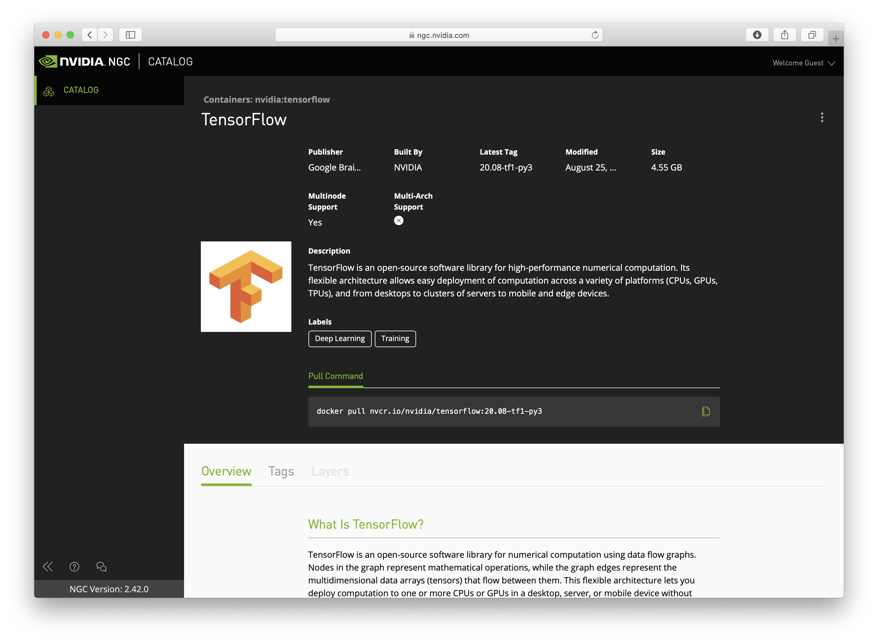 

Open the command line of your machine and paste the pull command into your command line. Execute the command to download the container.

$ docker pull nvcr.io/nvidia/pytorch:21.11-py3

The container starts downloading to your computer. A container image consists of many layers; all of them need to be pulled.

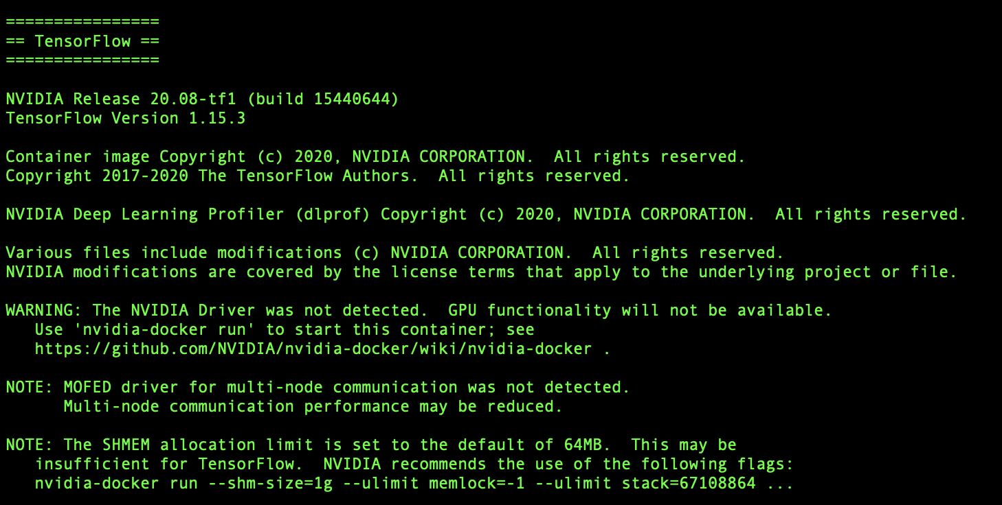
3. Run the TensorFlow container image

Once the container download is completed, run the following code in your command line to run and start the container:

$ docker run -it --gpus all -p 8888:8888 -v $PWD:/projects --network=host nvcr.io/nvidia/pytorch:21.11-py3

4. Install Jupyter lab and open a notebook

Within the container, run the following commands:

pip install torchvision==0.11.3 jupyterlab

jupyter lab --ip=0.0.0.0 --port=8888 --allow-root

Open up your favorite browser and enter: http://localhost:8888/?token=*yourtoken*.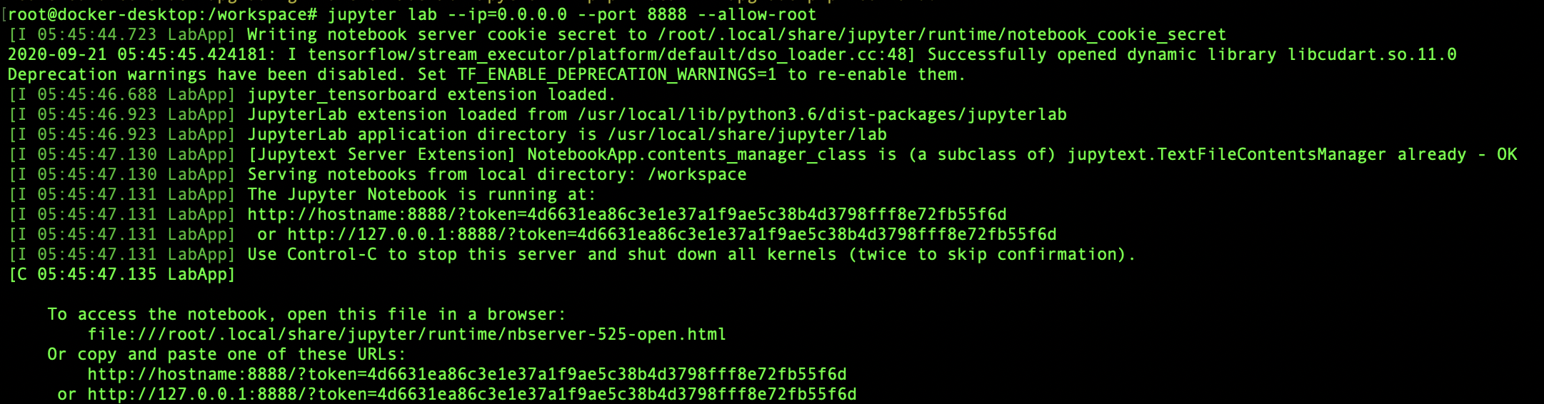

You should see the Jupyter Lab application. Click on the plus icon to launch a new Python 3 notebook. Follow the instructions regarding the image classification with the TensorFlow example provided in Part 2.

Now that you have your Docker engine installed and the PyTorch Container running, we need to fetch and prepare our training dataset. You'll see that coming up in Part 2 below.

Part 2: Data preparation

Note this Demo is based on NGC Docker image nvcr.io/nvidia/pytorch:21.11-py3

This notebook walks you through each step required to train a model using containers from the NGC catalog. We chose the GPU optimized PyTorch container as an example. The basics of working with docker containers apply to all NGC containers.

Here, I will show you how to:

• Download the xView Dataset
• How to convert labels to coco format
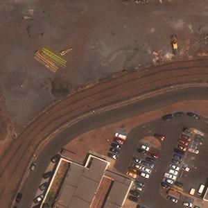
• How to conduct the preprocessing step, Tiling: slicing large satellite imagery into chunks
• How to upload to S3 bucket to support distributed training

Let's get started!

Pre-reqs, set up Jupyter Notebook environment using NGC container

Execute Docker run to create NGC environment for data preparation

Make sure to map host directory to Docker directory. You will use the host directory again to do the following:

• docker run --gpus all --ipc=host --ulimit memlock=-1 --ulimit stack=67108864 -v /home/ubuntu:/home/ubuntu -p 8008:8888 -it nvcr.io/nvidia/pytorch:21.11-py3 /bin/bash

Run Jupyter Notebook command within Docker container to access it on your local browser

• cd /home/ubuntu
• jupyter lab --ip=0.0.0.0 --port=8888 --NotebookApp.token='' --NotebookApp.password=''
• git clone https://github.com/interactivetech/e2e_blogposts.git

Download the xView dataset

The dataset you will be using is from the DIUx xView 2018 Challenge by U.S. National Geospatial-Intelligence Agency (NGA). You will need to create an account, agree to the terms and conditions, and download the dataset manually.

You can also download the dataset.

# run pip install to get the SAHI library
!pip install sahi scikit-image opencv-python-headless==4.5.5.64

# Example command to download train images with wget command, you will need to update the url as the token is expired"
!wget -O train_images.tgz "https://d307kc0mrhucc3.cloudfront.net/train_images.tgz?Expires=1680923794&Signature=pn0R9k3BpSukGEdjcNx7Kvs363HWkngK8sQLHxkDOqqkDAHSOCDBmAMAsBhYZ820uMpyu4Ynp1UAV60OmUURyvGorfIRaVF~jJO8-oqRVLeO1f24OGCQg7HratHNUsaf6owCb8XXy~3zaW15FcuORuPV-2Hr6Jxekwcdw9D~g4M2dLufA~qBfTLh3uNjWK5UCAMvyPz2SRLtvc3JLzGYq1eXiKh1dI9W0DyWXov3mVDpBdwS84Q21S2lVi24KJsiZOSJqozuvahydW2AuR~tbXTRbYtmAyPF9ZqT8ZCd9MLeKw2qQJjb7tvzaSZ0F9zPjm2RS8961bo6QoBVeo6kzA__&Key-Pair-Id=APKAIKGDJB5C3XUL2DXQ"

# Example command to download train images with wget command, you will need to update the url as the token is expired"
!wget -O train_labels.tgz "https://d307kc0mrhucc3.cloudfront.net/train_labels.tgz?Expires=1680923794&Signature=YEX~4gioZ7J0pAjEPx7BjJfnOa2j412mx2HlStlqa0cHj-T0T21vo17S8Fs71DXgPlZ5qnIre2-icc7wQ~EuQV-HL1ViS8qH1Aubgj9i0pnHZL07ktiyulX7QStOLywxJ7bOOmQ37iFF~-OcJW3MZfQCTWrP~LdlZMmXz0yGs5WEIYeMyvfUfIhGvrpHcJ14Z3czasSMeOKfwdQsUJoRcFTbmlbZk98IVeEWjmnGTfxGbPBdMmQ96XdT4NohggtzGdqeZhGNfwm7dKGSUbXvGCoFe~fIjBz0~5BvB6rNIaMaFuBA6aGTbCLeG8FlvijcECouhZdMTHmQUlgtSlZjGw__&Key-Pair-Id=APKAIKGDJB5C3XUL2DXQ"

# unzip images and labels from /home/ubuntu/e2e_blogposts/ngc_blog
!tar -xf train_images.tgz -C xview_dataset/

# unzip labels from /home/ubuntu/e2e_blogposts/ngc_blog directory 
!tar -xf train_labels.tgz -C xview_dataset/

1. Convert TIF to RGB

# Here loop through all the images and convert them to RGB, this is important for tiling the images and training with pytorch
# will take about an hour to complete
!python data_utils/tif_2_rgb.py --input_dir xview_dataset/train_images \
  --out_dir xview_dataset/train_images_rgb/

2. How to convert labels to COCO format

Run a script to convert the dataset labels from .geojson format to COCO format. Read more details about the COCO format at this link.

The result will be two files (in COCO formal) generated train.json and val.json

# make sure train_images_dir is pointing to the .tif images
!python data_utils/convert_geojson_to_coco.py --train_images_dir xview_dataset/train_images/ \
  --train_images_dir_rgb xview_dataset/train_images_rgb/ \
  --train_geojson_path xview_dataset/xView_train.geojson \
  --output_dir xview_dataset/ \
  --train_split_rate 0.75 \
  --category_id_remapping data_utils/category_id_mapping.json \
  --xview_class_labels data_utils/xview_class_labels.txt

3. Slicing/Tiling the dataset

Here, you will be using the SAHI library to slice our large satellite images. Satellite images can be up to 50k^2 pixels in size, which wouldn't fit in GPU memory. You can alleviate this problem by slicing the image.

!python data_utils/slice_coco.py --image_dir xview_dataset/train_images_rgb/ \
  --train_dataset_json_path xview_dataset/train.json \
  --val_dataset_json_path xview_dataset/val.json \
  --slice_size 300 \
  --overlap_ratio 0.2 \
  --ignore_negative_samples True \
  --min_area_ratio 0.1 \
  --output_train_dir xview_dataset/train_images_rgb_no_neg/ \
  --output_val_dir xview_dataset/val_images_rgb_no_neg/

4. Upload to S3 bucket to support distributed training

Now, you can upload your exported data to a publicly accessible AWS S3 bucket. For a large-scale distributed experiment, this will enable you to access the dataset without installing the dataset on the device. View Determined Documentation and AWS instructions to learn how to upload your dataset to an S3 bucket. Review the S3Backend class in data.py

Once you create an S3 bucket that is publicly accessible, here are example commands to upload the preprocessed dataset to S3:

• aws s3 cp --recursive xview_dataset/train_sliced_no_neg/ s3://determined-ai-xview-coco-dataset/train_sliced_no_neg
• aws s3 cp --recursive xview_dataset/val_sliced_no_neg/ s3://determined-ai-xview-coco-dataset/val_sliced_no_neg

Now that the satellite imagery data is in an S3 bucket and is prepped for distributed training, you can progress to model training and inferencing via the NGC container.

Part 3: End-to-End example training object detection model using NVIDIA PyTorch container from NGC

Training and inference via NGC Container

This notebook walks you through each step to train a model using containers from the NGC Catalog. I chose the GPU-optimized PyTorch container for this example. The basics of working with Docker containers apply to all NGC containers.

We will show you how to:

• Execute training an object detection model on satellite imagery using TensorFlow and Jupyter Notebook
• Run inference on a trained object detection model using the SAHI library

Note this object detection demo is based on this PyTorch repo and ngc docker image nvcr.io/nvidia/pytorch:21.11-py3

It is assumed that, by now, you have completed step 2 of dataset preprocessing and have your tiled satellite imagery dataset completed and in the local directory train_images_rgb_no_neg/train_images_300_02

Let's get started!

Execute Docker run to create NGC environment for data prep

Make sure to map host directory to Docker directory. You will use the host directory again to:

• docker run --gpus all --ipc=host --ulimit memlock=-1 --ulimit stack=67108864 -v /home/ubuntu:/home/ubuntu -p 8008:8888 -it nvcr.io/nvidia/pytorch:21.11-py3 /bin/bash

Run Jupyter Notebook command within Docker container to access it on your local browser

• cd /home/ubuntu
• jupyter lab --ip=0.0.0.0 --port=8888 --NotebookApp.token='' --NotebookApp.password=''

%%capture
!pip install cython pycocotools matplotlib terminaltables

TLDR; Run training job on 4 GPUs

The below cell will run a multi-gpu training job. This job will train an object detection model (faster-rcnn) on a dataset of satellite imagery images that contain 61 classes of objects.

• Change nproc_per_node argument to specify the number of GPUs available on your server

!torchrun --nproc_per_node=4 detection/train.py\
    --dataset coco --data-path=xview_dataset/ --model fasterrcnn_resnet50_fpn --epochs 26\
    --lr-steps 16 22 --aspect-ratio-group-factor 3

1. Object detection on satellite imagery with PyTorch (single GPU)

Follow and run the code to train a Faster RCNN FPN (Resnet50 backbone) that classifies images of clothing.

import sys
sys.path.insert(0,'detection')

# Import python dependencies
import datetime
import os
import time

import torch
import torch.utils.data
import torchvision
import torchvision.models.detection
import torchvision.models.detection.mask_rcnn

from coco_utils import get_coco, get_coco_kp

from group_by_aspect_ratio import GroupedBatchSampler, create_aspect_ratio_groups
from engine import train_one_epoch, evaluate

import presets
import utils
from coco_utils import get_coco, get_coco_kp
from train import get_dataset, get_transform
from group_by_aspect_ratio import GroupedBatchSampler, create_aspect_ratio_groups
from engine import train_one_epoch, evaluate
from models import build_frcnn_model
from PIL import Image
from torchvision.models.detection.faster_rcnn import FastRCNNPredictor
from collections import OrderedDict
from tqdm import tqdm
from vis_utils import load_determined_state_dict, visualize_pred, visualize_gt, predict
import numpy as np

import matplotlib.pyplot as plt

output_dir='output'
data_path='xview_dataset/'
dataset_name='coco'
model_name='fasterrcnn_resnet50_fpn'
device='cpu'
batch_size=8
epochs=26
workers=4
lr=0.02
momentum=0.9
weight_decay=1e-4
lr_scheduler='multisteplr'
lr_step_size=8
lr_steps=[16, 22]
lr_gamma=0.1
print_freq=20
resume=False
start_epoch=0
aspect_ratio_group_factor=3
rpn_score_thresh=None
trainable_backbone_layers=None
data_augmentation='hflip'
pretrained=True
test_only=False
sync_bn=False

# Import the dataset.
# Data loading code
print("Loading data")

dataset, num_classes = get_dataset(dataset_name, "train", get_transform(True, data_augmentation),
                                   data_path)
dataset_test, _ = get_dataset(dataset_name, "val", get_transform(False, data_augmentation), data_path)
print(dataset.num_classes)
print("Creating data loaders")
train_sampler = torch.utils.data.RandomSampler(dataset)
test_sampler = torch.utils.data.SequentialSampler(dataset_test)
group_ids = create_aspect_ratio_groups(dataset, k=aspect_ratio_group_factor)
train_batch_sampler = GroupedBatchSampler(train_sampler, group_ids, batch_size)
train_batch_sampler = torch.utils.data.BatchSampler(
            train_sampler, batch_size, drop_last=True)

data_loader = torch.utils.data.DataLoader(
    dataset, batch_sampler=train_batch_sampler, num_workers=workers,
    collate_fn=utils.collate_fn)

data_loader_test = torch.utils.data.DataLoader(
    dataset_test, batch_size=1,
    sampler=test_sampler, num_workers=0,
    collate_fn=utils.collate_fn)

# Getting three examples from the test dataset
inds_that_have_boxes = []
test_images = list(data_loader_test)
for ind,(im,targets) in tqdm(enumerate(test_images),total=len(list(data_loader_test))):
    # print(ind,targets)
    if targets[0]['boxes'].shape[0]>0:
        # print(targets[0]['boxes'].shape[0])
        # print(ind,targets)
        inds_that_have_boxes.append(ind)

images_t_list=[]
targets_t_list=[]
for ind in tqdm(range(3)):
    im,targets = test_images[ind]
    images_t_list.append(im[0])
    targets_t_list.append(targets[0])

# Let's have a look at one of the images. The following code visualizes the images using the matplotlib library.
im = Image.fromarray((255.*images_t_list[0].cpu().permute((1,2,0)).numpy()).astype(np.uint8))
plt.imshow(im)
plt.show()

# Let's look again at the first three images, but this time with the class names.

for i,t in zip(images_t_list,targets_t_list):
    im = Image.fromarray((255.*i.cpu().permute((1,2,0)).numpy()).astype(np.uint8))
    plt.imshow(im)
    plt.show()
    im = visualize_gt(i,t)
    plt.imshow(im)
    plt.show()

# Let's build the model:
print("Creating model")
print("Number of classes: ",dataset.num_classes)
model = build_frcnn_model(num_classes=dataset.num_classes)
_=model.to('cpu')

# Compile the model:
# Define loss function, optimizer, and metrics.
params = [p for p in model.parameters() if p.requires_grad]
optimizer = torch.optim.SGD(
    params, lr=lr, momentum=momentum, weight_decay=weight_decay)

lr_scheduler = lr_scheduler.lower()
if lr_scheduler == 'multisteplr':
    lr_scheduler = torch.optim.lr_scheduler.MultiStepLR(optimizer, 
                                                        milestones=lr_steps, 
                                                        gamma=lr_gamma)
elif lr_scheduler == 'cosineannealinglr':
    lr_scheduler = torch.optim.lr_scheduler.CosineAnnealingLR(optimizer, T_max=epochs)
else:
    raise RuntimeError("Invalid lr scheduler '{}'. Only MultiStepLR and CosineAnnealingLR "
                       "are supported.".format(args.lr_scheduler))

# Train the model:
# Let's train 1 epoch. After every epoch, training time, loss, and accuracy will be displayed.
print("Start training")
start_time = time.time()
for epoch in range(start_epoch, epochs):
    train_one_epoch(model, optimizer, data_loader, device, epoch, print_freq)
    lr_scheduler.step()
    if output_dir:
        checkpoint = {
            'model': model.state_dict(),
            'optimizer': optimizer.state_dict(),
            'lr_scheduler': lr_scheduler.state_dict(),
            'args': args,
            'epoch': epoch
        }
        utils.save_on_master(
            checkpoint,
            os.path.join(output_dir, 'model_{}.pth'.format(epoch)))
        utils.save_on_master(
            checkpoint,
            os.path.join(output_dir, 'checkpoint.pth'))

    # evaluate after every epoch
    evaluate(model, data_loader_test, device=device)

total_time = time.time() - start_time
total_time_str = str(datetime.timedelta(seconds=int(total_time)))
print('Training time {}'.format(total_time_str))

def build_frcnn_model2(num_classes):
    print("Loading pretrained model...")
    # load an detection model pre-trained on COCO
    model = torchvision.models.detection.fasterrcnn_resnet50_fpn(pretrained=True)

    # get the number of input features for the classifier
    in_features = model.roi_heads.box_predictor.cls_score.in_features
    # replace the pre-trained head with a new one
    model.roi_heads.box_predictor = FastRCNNPredictor(in_features, num_classes)
    model.min_size=800
    model.max_size=1333
    # RPN parameters
    model.rpn_pre_nms_top_n_train=2000
    model.rpn_pre_nms_top_n_test=1000
    model.rpn_post_nms_top_n_train=2000
    model.rpn_post_nms_top_n_test=1000
    model.rpn_nms_thresh=1.0
    model.rpn_fg_iou_thresh=0.7
    model.rpn_bg_iou_thresh=0.3
    model.rpn_batch_size_per_image=256
    model.rpn_positive_fraction=0.5
    model.rpn_score_thresh=0.05
    # Box parameters
    model.box_score_thresh=0.0
    model.box_nms_thresh=1.0
    model.box_detections_per_img=500
    model.box_fg_iou_thresh=1.0
    model.box_bg_iou_thresh=1.0
    model.box_batch_size_per_image=512
    model.box_positive_fraction=0.25
    return model

# Let's see how the model performs on the test data:
model = build_frcnn_model2(num_classes=61)
ckpt = torch.load('model_8.pth',map_location='cpu')
model.load_state_dict(ckpt['model'])
_=model.eval()

_=predict(model,images_t_list,targets_t_list)

In the next part of this blog post, I will show you how to scale your model training using using distributed training within HPE Machine Learning Development Environment & System.

Part 4: Training on HPE Machine Learning Development & System

HPE Machine Learning Development Environment is a training platform software that reduces complexity for ML researchers and helps research teams collaborate. HPE combines this incredibly powerful training platform with best-of-breed hardware and interconnect in HPE Machine Learning Development System, an AI turnkey solution that will be used for the duration of the tutorial.

This notebook walks you through the commands to run the same training you did in stepin Step 3, but using the HPE Machine Learning Development Environment together with the PyTorchTrial API. All the code is configured to run out of the box. The main change is defining a class ObjectDetectionTrial(PyTorchTrial) to incorporate the model, optimizer, dataset, and other training loop essentials. You can view implementation details by looking at determined_files/model_def.py

Here, I will show you how to:

• Run a distributed training experiment
• Run a distributed hyperparameter search

Note: This notebook was tested on a deployed HPE Machine Learning Development System cluster, running HPE Machine Learning Development Environment (0.21.2-dev0).

Let's get started!

Pre-req: Run startup-hook.sh

This script will install some python dependencies, and install dataset labels needed when loading the xView dataset:

## Temporary disable for Grenoble Demo
wget "https://determined-ai-xview-coco-dataset.s3.us-west-2.amazonaws.com/train_sliced_no_neg/train_300_02.json"
mkdir /tmp/train_sliced_no_neg/
mv train_300_02.json /tmp/train_sliced_no_neg/train_300_02.json 
wget "https://determined-ai-xview-coco-dataset.s3.us-west-2.amazonaws.com/val_sliced_no_neg/val_300_02.json"
mkdir /tmp/val_sliced_no_neg
mv val_300_02.json /tmp/val_sliced_no_neg/val_300_02.json

Note that completing this tutorial requires you to upload your dataset from Step 2 into a publicly accessible S3 bucket. This will enable for a large scale distributed experiment to have access to the dataset without installing the dataset on device. View Determined Documentation and AWS instructions to learn how to upload your dataset to an S3 bucket. Review the S3Backend class in data.py

When you define your S3 bucket and uploaded your dataset, make sure to change the TARIN_DATA_DIR in build_training_data_loader with the defined path in the S3 bucket.

def build_training_data_loader(self) -> DataLoader:
    # CHANGE TRAIN_DATA_DIR with different path on S3 bucket
    TRAIN_DATA_DIR='determined-ai-xview-coco-dataset/train_sliced_no_neg/train_images_300_02/'

    dataset, num_classes = build_xview_dataset(image_set='train',args=AttrDict({
                                            'data_dir':TRAIN_DATA_DIR,
                                            'backend':'aws',
                                            'masks': None,
                                            }))
    print("--num_classes: ",num_classes)

    train_sampler = torch.utils.data.RandomSampler(dataset)

    data_loader = DataLoader(
                             dataset, 
                             batch_sampler=None,
                             shuffle=True,
                             num_workers=self.hparams.num_workers, 
                             collate_fn=unwrap_collate_fn)
    print("NUMBER OF BATCHES IN COCO: ",len(data_loader))# 59143, 7392 for mini coco

!bash demos/xview-torchvision-coco/startup-hook.sh

Define environment variable DET_MASTER and login in terminal

Run the below commands in a terminal, and complete logging into the Determined cluster by changing to your username.

• export DET_MASTER=10.182.1.43
• det user login <username>

Define Determined experiment

In Determined, a trial is a training task that consists of a dataset, a deep learning model, and values for all of the model’s hyperparameters. An experiment is a collection of one or more trials: an experiment can either train a single model (with a single trial), or can train multiple models via a hyperparameter sweep a user-defined hyperparameter space.

Here is what a configuration file looks like for a distributed training experiment.

Below is what the determined_files/const-distributed.yaml contents look like. slots_per_trial: 8 defines that we will use 8 GPUs for this experiment.

Edit the change the workspace and project settings in the determined_files/const-distributed.yaml file

name: resnet_fpn_frcnn_xview_dist_warmup
workspace: <WORKSPACE_NAME>
project: <PROJECT_NAME>
profiling:
 enabled: true
 begin_on_batch: 0
 end_after_batch: null
hyperparameters:
    lr: 0.01
    momentum: 0.9
    global_batch_size: 128
    # global_batch_size: 16
    weight_decay: 1.0e-4
    gamma: 0.1
    warmup: linear
    warmup_iters: 200
    warmup_ratio: 0.001

    step1: 18032 # 14 epochs: 14*1288 == 18,032
    step2: 19320 # 15 epochs: 15*1288 == 19,320
    model: fasterrcnn_resnet50_fpn
    # Dataset
    dataset_file: coco
    backend: aws # specifiy the backend you want to use.  one of: gcs, aws, fake, local
    data_dir: determined-ai-coco-dataset # bucket name if using gcs or aws, otherwise directory to dataset
    masks: false
    num_workers: 4
    device: cuda
environment:
    image: determinedai/environments:cuda-11.3-pytorch-1.10-tf-2.8-gpu-mpi-0.19.10
    environment_variables:                                                                          
        - NCCL_DEBUG=INFO                                                                           
        # You may need to modify this to match your network configuration.                          
        - NCCL_SOCKET_IFNAME=ens,eth,ib
bind_mounts:
    - host_path: /tmp
      container_path: /data
      read_only: false
scheduling_unit: 400
min_validation_period:
    batches: 1288 # For training

searcher:
  name: single
  metric: mAP
  smaller_is_better: true
  max_length:
    batches: 38640 # 30*1288 == 6440# Real Training
records_per_epoch: 1288
resources:
    slots_per_trial: 8
    shm_size: 2000000000
max_restarts: 0

entrypoint: python3 -m determined.launch.torch_distributed --trial model_def:ObjectDetectionTrial

# Run the below cell to kick off an experiment
!det e create determined_files/const-distributed.yaml determined_files/

Preparing files to send to master... 237.5KB and 36 files
Created experiment 77

Launching a distributed hyperparameter search experiment

To implement an automatic hyperparameter tuning experiment, define the hyperparameter space, e.g. by listing the decisions that may impact model performance. You can specify a range of possible values in the experiment configuration for each hyperparameter in the search space.

View the x.yaml file that defines a hyperparameter search where the model architecture that achieves the best performance on the dataset is found..

name: xview_frxnn_search
workspace: Andrew
project: Xview FasterRCNN
profiling:
 enabled: true
 begin_on_batch: 0
 end_after_batch: null
hyperparameters:
    lr: 0.01
    momentum: 0.9
    global_batch_size: 128
    weight_decay: 1.0e-4
    gamma: 0.1
    warmup: linear
    warmup_iters: 200
    warmup_ratio: 0.001
    step1: 18032 # 14 epochs: 14*1288 == 18,032
    step2: 19320 # 15 epochs: 15*1288 == 19,320
    model:
      type: categorical
      vals: ['fasterrcnn_resnet50_fpn','fcos_resnet50_fpn', 'ssd300_vgg16','ssdlite320_mobilenet_v3_large','resnet152_fasterrcnn_model','efficientnet_b4_fasterrcnn_model','convnext_large_fasterrcnn_model','convnext_small_fasterrcnn_model']

    # Dataset
    dataset_file: coco
    backend: aws # specifiy the backend you want to use.  one of: gcs, aws, fake, local
    data_dir: determined-ai-coco-dataset # bucket name if using gcs or aws, otherwise directory to dataset
    masks: false
    num_workers: 4

    device: cuda
environment:
    environment_variables:                                                                          
        - NCCL_DEBUG=INFO                                                                           
        # You may need to modify this to match your network configuration.                          
        - NCCL_SOCKET_IFNAME=ens,eth,ib
bind_mounts:
    - host_path: /tmp
      container_path: /data
      read_only: false
scheduling_unit: 400
# scheduling_unit: 40
min_validation_period:
    batches: 1288 # For Real training
searcher:
  name: grid
  metric: mAP
  smaller_is_better: false
  max_length:
    batches: 51520 # 50*1288 == 51520# Real Training

records_per_epoch: 1288
resources:
    # slots_per_trial: 16
    slots_per_trial: 8
    shm_size: 2000000000
max_restarts: 0

entrypoint: python3 -m determined.launch.torch_distributed --trial model_def:ObjectDetectionTrial

# Run the below cell to run a hyperparameter search experiment
!det e create determined_files/const-distributed-search.yaml determined_files/

Preparing files to send to master... 312.2KB and 40 files
Created experiment 79

Load checkpoint of trained experiment

Replace the <EXP_ID> and run the below cells with the experiment ID once the experiment is completed.

from determined_files.utils.model import build_frcnn_model
from utils import load_model_from_checkpoint
from determined.experimental import Determined,client

experiment_id = 76
MODEL_NAME = "xview-fasterrcnn"
checkpoint = client.get_experiment(experiment_id).top_checkpoint(sort_by="mAP", smaller_is_better=False)
print(checkpoint.uuid)
loaded_model = load_model_from_checkpoint(checkpoint)

Now that you have a checkpoint from the trained object detection model, you can deploy it to Kserve to run inference and predictions.

Part 5: Deploying trained model on Kserve

This notebook walks you each step to deploy a custom object detection model on KServe.

Here, I will show you how to:

• Install Kserve natively using Kind and Knative
• Create a Persistent Volume Claim for local model deployment
• Preparing custom model for Kserve inference
• Deploying model using a KServe InferenceService
• Complete a sample request and plot predictions

Note: This notebook was tested on a Linux-based machine with Nvidia T4 GPUs. We also assume Docker is installed in your Linux system/environment

Let's get started!

Pre-reqs: Setting up Python and Jupyter Lab environment

Run the below commands to set up a Python virtual environment, and install all the Python packages needed for this tutorial

sudo apt-get update && sudo apt-get  install python3.8-venv
python3 -m venv kserve_env
source kserve_env/bin/activate
pip install kserve jupyterlab torch-model-archiver
pip install torch==1.11.0 torchvision==0.12.0 matplotlib
jupyter lab --ip=0.0.0.0 \
  --port=8008 \
  --NotebookApp.token='' \
  --NotebookApp.password=''

Install Kserve natively using Kind and Knative

Install Kind

Open a terminal and run the following bash commands to install a Kubernetes cluster using Kind:

• curl -Lo ./kind https://kind.sigs.k8s.io/dl/v0.18.0/kind-linux-amd64
• chmod +x ./kind
• sudo mv ./kind /usr/local/bin/kind

After running these commands, create a cluster by running the command: kind create cluster

Install Kubectl

Run the following bash commmands in a terminal to to install the kubectl runtime:

• curl -LO "https://dl.k8s.io/release/$(curl -L -s https://dl.k8s.io/release/stable.txt)/bin/linux/amd64/kubectl"
• curl -LO "https://dl.k8s.io/$(curl -L -s https://dl.k8s.io/release/stable.txt)/bin/linux/amd64/kubectl.sha256"
• sudo install -o root -g root -m 0755 kubectl /usr/local/bin/kubectl

Install Kserve

Run this bash script to install KServe onto our default Kubernetes cluster, note this will install the following artifacts:

• ISTIO_VERSION=1.15.2, KNATIVE_VERSION=knative-v1.9.0, KSERVE_VERSION=v0.9.0-rc0, CERT_MANAGER_VERSION=v1.3.0
• bash e2e_blogposts/ngc_blog/kserve_utils/bash_scripts/kserve_install.sh

Patch domain for local connection to KServe cluster/environment

Run this command to patch your cluster when you want to connect to your cluster on the same machine:

kubectl patch cm config-domain --patch '{"data":{"example.com":""}}' -n knative-serving

Run port forwarding to access KServe cluster

• INGRESS_GATEWAY_SERVICE=$(kubectl get svc --namespace istio-system --selector="app=istio-ingressgateway" --output jsonpath='{.items[0].metadata.name}')
• kubectl port-forward --namespace istio-system svc/${INGRESS_GATEWAY_SERVICE} 8080:80

Make sure to open a new terminal to continue the configuration.

Create a persistent volume claim for local model deployment

You will be creating a persistent volume claim to host and access the PyTorch-based object detection model locally. A persistent volume claim requires three k8s artifacts:

• A persistent volume
• A persistent volume claim
• A k8s pod that connects the PVC to be accessed by other k8s resources

Creating a persistent volume and persistent volume claim

Below is the yaml definition that defines the Persistent Volume (PV) and a PersistentVolumeClaim (PVC). We already created a file that defines this PV in k8s_files/pv-and-pvc.yaml

apiVersion: v1
kind: PersistentVolume
metadata:
  name: task-pv-volume
  labels:
    type: local
spec:
  storageClassName: manual
  capacity:
    storage: 2Gi
  accessModes:
    - ReadWriteOnce
  hostPath:
    path: "/home/ubuntu/mnt/data"
---
apiVersion: v1
kind: PersistentVolumeClaim
metadata:
  name: task-pv-claim
spec:
  storageClassName: manual
  accessModes:
    - ReadWriteOnce
  resources:
    requests:
      storage: 1Gi

To create the PV and PVC, run the command: kubectl apply -f k8s_files/pv-and-pvc.yaml

Create k8s pod to access PVC

Below is the yaml definition that defines the k8s Pod that mounts the PersistentVolumeClaim (PVC). We already created a file that defines this PV in k8s_files/model-store-pod.yaml

apiVersion: v1
kind: Pod
metadata:
  name: model-store-pod
spec:
  volumes:
    - name: model-store
      persistentVolumeClaim:
        claimName: task-pv-claim
  containers:
    - name: model-store
      image: ubuntu
      command: [ "sleep" ]
      args: [ "infinity" ]
      volumeMounts:
        - mountPath: "/pv"
          name: model-store
      resources:
        limits:
          memory: "1Gi"
          cpu: "1"

To create the Pod, run the command: kubectl apply -f k8s_files/model-store-pod.yaml

Preparing custom model for Kserve inference

Here we will complete some preparation steps to deploy a trained custom FasterRCNN Object Detection model using KServe. A pre-requisite is to download a checkpoint from a determined experiement. You can read this tutorial on how to download a checkpoint using the Determined CLI. For this tutorial, you can download an already prepared checkpoint using the following bash command:

• wget -O kserve_utils/torchserve_utils/trained_model.pth https://determined-ai-xview-coco-dataset.s3.us-west-2.amazonaws.com/trained_model.pth

Stripping the checkpoint of the optimizer state dictionary

Checkpoints created from a Determined experiment will save both the model parameters and the optimizer parameters. You will need to strip the checkpoint of all parameters except the model parameters for inference. Run the bash command to generate train_model_stripped.pth:

Run the below command in a terminal:

python kserve_utils/torchserve_utils/strip_checkpoint.py --ckpt-path kserve_utils/torchserve_utils/trained_model.pth \
  --new-ckpt-name kserve_utils/torchserve_utils/trained_model_stripped.pth

Run TorchServe Export to create .mar file

Run the below command to export the PyTorch checkpoint into a .mar file that is required for torchserve inference. The Kserve InferenceService will automatically deploy a Pod with a docker image that support TorchServe inferencing.

torch-model-archiver --model-name xview-fasterrcnn \
  --version 1.0 \
  --model-file kserve_utils/torchserve_utils/model-xview.py \
  --serialized-file kserve_utils/torchserve_utils/trained_model_stripped.pth \
  --handler kserve_utils/torchserve_utils/fasterrcnn_handler.py \
  --extra-files kserve_utils/torchserve_utils/index_to_name.json

After command finishes, run the command to move the file to our prepared model-store/ directory:

• cp xview-fasterrcnn.mar kserve_utils/torchserve_utils/model-store -v

Copy config/ and model-store/ folders to the K8S PVC Pod

This is the directory structure needed to prepare your custom PyTorch model for KServe inferencing:

├── config
│   └── config.properties
├── model-store
│   ├── properties.json
│   └── xview-fasterrcnn.mar

What the config.properties file looks like

inference_address=http://0.0.0.0:8085
management_address=http://0.0.0.0:8085
metrics_address=http://0.0.0.0:8082
grpc_inference_port=7070
grpc_management_port=7071
enable_metrics_api=true
metrics_format=prometheus
number_of_netty_threads=4
job_queue_size=10
enable_envvars_config=true
install_py_dep_per_model=true
model_store=/mnt/models/model-store
model_snapshot={"name": "startup.cfg","modelCount": 1,"models": {"xview-fasterrcnn": {"1.0": {"defaultVersion": true,"marName": "xview-fasterrcnn.mar","serialized-file":"trained_model_stripped.pth","extra-files":"index_to_name.json","handler":"fasterrcnn_handler.py","minWorkers": 1,"maxWorkers": 5,"batchSize": 1,"maxBatchDelay": 100,"responseTimeout": 120}}}}

What the properties.json looks like

[
    {
    "model-name": "xview-fasterrcnn",
    "version": "1.0",
    "model-file": "",
    "serialized-file": "trained_model_stripped.pth",
    "extra-files": "index_to_name.json",
    "handler": "fasterrcnn_handler.py",
    "min-workers" : 1,
    "max-workers": 3,
    "batch-size": 1,
    "max-batch-delay": 100,
    "response-timeout": 120,
    "requirements": ""
  }
]

Note that there is a config/ folder that includes a config.properties. This defines A. There is also a model-store/ directory that contains are exported models and a properties.json file. You will need this file for B.

Now, run several kubectl commands to copy over these folders into your Pod and into the PVC defined directory.

• kubectl cp kserve_utils/torchserve_utils/config/ model-store-pod:/pv/config/
• kubectl cp kserve_utils/torchserve_utils/model-store/ model-store-pod:/pv/model-store/

Run these commands to verify the contents have been copied over to the pod.

• kubectl exec --tty model-store-pod -- ls /pv/config
• kubectl exec --tty model-store-pod -- ls /pv/model-store

Deploying a model using a KServe InferenceService

Create Inference Service

Below is the yaml definition that defines the KServe InferenceService that deploys models stored in the PVC. A file that defines this PV has already been created in k8s_files/torch-kserve-pvc.yaml

apiVersion: "serving.kserve.io/v1beta1"
kind: "InferenceService"
metadata:
  name: "torchserve"
spec:
  predictor:
    pytorch:
      storageUri: pvc://task-pv-claim/

To create the Pod, run the command: kubectl apply -f kserve_utils/k8s_files/torch-kserve-pvc.yaml

• After running the previous command kubectl get inferenceservice, you should see that the inferenceservice is not loaded yet
• Keep running the command every minute until you see the InferenceService loaded (view screenshot below of example)
• Next, run command kubectl get pods to get underlying pod that is running inference service. Copy the pod name (example seen in screenshot)
• Finally run command: kubectl logs -f <POD_NAME> to see the logs and if the model was successfully loaded.

Complete a sample request and plot predictions

import json
import requests
import base64
from PIL import Image
from PIL import ImageDraw
import matplotlib.pyplot as plt

filename='kserve_utils/torchserve_utils/example_img.jpg'
im = Image.open(filename)

Here is the test image that will be sent to the deployed model.

im

Now, encode the image into the base64 binary format.

image = open(filename, 'rb')  # open binary file in read mode
image_read = image.read()
image_64_encode = base64.b64encode(image_read)
bytes_array = image_64_encode.decode('utf-8')
request = {
  "instances": [
    {
      "data": bytes_array
    }
  ]
}
result_file = "{filename}.{ext}".format(filename=str(filename).split(".")[0], ext="json")
print("Result File: ",result_file)
with open(result_file, 'w') as outfile:
    json.dump(request, outfile, indent=4, sort_keys=True)

Result File:  kserve_utils/torchserve_utils/example_img.json

Now you can submit the image to the deployed endpoint and visualize the predictions!

headers = {
    "Host": "torchserve.default.example.com"
}

data = open(result_file)
response = requests.post('http://localhost:8080/v1/models/xview-fasterrcnn:predict', headers=headers, data=data)

resp = json.loads(response.content)

print("Number of Predictions: ", len(resp['predictions'][0]))

Number of Predictions:  95

draw = ImageDraw.Draw(im)

for pred in resp['predictions'][0]:
    assert len(list(pred.keys())) == 2
    cl_name = list(pred.keys())[0]
    bboxes = pred[cl_name]
    # print(cl_names)
    # print(bboxes)
    # print("score: ",pred['score'])
    if pred['score'] > 0.4:
        # bboxes = [int(i) for i in bboxes]
        # print(bboxes[0],type(bboxes[0]))
        draw.rectangle([bboxes[0],bboxes[1],bboxes[2],bboxes[3]],outline=(255,0,0),fill=None,width=1)
        draw.text([bboxes[0],bboxes[1]-10],"{} :{:.2f}".format(cl_name,pred['score']),fill=(250,0,0))

Here, you can see the model predictions overlaid onto the input image.

plt.figure(figsize=(12,12))
plt.imshow(im)

<matplotlib.image.AxesImage at 0x7ff6341ccf10>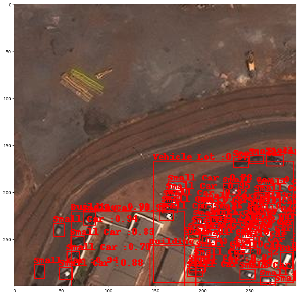

Conclusion

There are numerous ways to get started with end-to-end ML model training with HPE. You can find the full example on GitHub here To get started with Determined AI’s open source model training platform, visit the Documentation page.

If you’re ready to begin your ML journey with HPE, we’re excited to help you get started! HPE Machine Learning Development Environment comes with premium HPE support, which you can read more about here.

HPE also offers a purpose-built, turnkey AI infrastructure for model development and training at scale. Get in touch with us about HPE Machine Learning Development System here.