Analyzing Flight Delays with Apache Spark GraphFrames and MapR Database
December 16, 2020Editor’s Note: MapR products and solutions sold prior to the acquisition of such assets by Hewlett Packard Enterprise Company in 2019, may have older product names and model numbers that differ from current solutions. For information about current offerings, which are now part of HPE Ezmeral Data Fabric, please visit https://www.hpe.com/us/en/software/data-fabric.html
Original Post Information:
"authorDisplayName": "Carol McDonald",
"publish": "2018-11-16T07:00:00.000Z",
"tags": "nosql"
Apache Spark GraphX made it possible to run graph algorithms within Spark. GraphFrames integrates GraphX and DataFrames and makes it possible to perform Graph pattern queries without moving data to a specialized graph database.
This blog will help you get started using Apache Spark GraphFrames Graph Algorithms and Graph Queries with MapR Database JSON document database. We will begin with an overview of Graph and GraphFrames concepts, then we will analyze a real flight dataset for January-August 2018 stored in a MapR Database table.
Graphs provide a powerful way to analyze the connections in a Dataset. GraphX is the Apache Spark component for graph-parallel and data-parallel computations, built upon a branch of mathematics called graph theory. It is a distributed graph processing framework that sits on top of the Spark core. GraphX brings the speed and scalability of parallel, iterative processing to graphs for big datasets. It partitions graphs that are too large to fit in the memory of a single computer among multiple computers in a cluster. In addition, GraphX partitions vertices independently of edges, which avoids the load imbalance often suffered when putting all the edges for a vertex onto a single machine.
With Spark 2.0 and later versions, big improvements were implemented to make Spark easier to program and execute faster: Spark SQL and the Dataset/DataFrame APIs provide ease of use, space efficiency, and performance gains with Spark SQL's optimized execution engine. GraphFrames extends Spark GraphX to provide the DataFrame API, making the analysis easier to use, more efficient, and simplifying data pipelines.
Overview of Some Graph Concepts
A graph is a mathematical structure used to model relations between objects. A graph is made up of vertices and edges that connect them. The vertices are the objects, and the edges are the relationships between them.
A regular graph is a graph where each vertex has the same number of edges. An example of a regular graph is Facebook friends. If Ted is a friend of Carol, then Carol is also a friend of Ted.

A directed graph is a graph where the edges have a direction associated with them. An example of a directed graph is a Twitter follower. Carol can follow Oprah without implying that Oprah follows Carol.

GraphFrame Property Graph
Spark GraphFrames support graph computation with a distributed property graph. A property graph is a directed multigraph, which can have multiple edges in parallel. Every edge and vertex has user-defined properties associated with it. The parallel edges allow multiple relationships between the same vertices.

With GraphFrames, vertices and edges are represented as DataFrames, which adds the advantages of querying with Spark SQL and support for DataFrame data sources like Parquet, JSON, CSV, and also MapR Database with the MapR Database Spark Connector.
Graph Algorithms verses Graph Queries
Graph analysis comes in two forms: graph algorithms and graph pattern queries. Let’s look at an example of each and how GraphFrames integrates the two.
PageRank Graph Algorithm
The breakthrough for the creators of the Google search engine was to create the PageRank graph algorithm, which represents pages as nodes and links as edges and measures the importance of a page by the number and rank of linking pages, plus the number and rank of each of the linking pages. The PageRank algorithm is useful for measuring the importance of a vertex in a graph. Example of this could be a Twitter tweeter with lots of important followers or an airport with lots of connections to other airports with lots of connections.

Many graph algorithms such as PageRank, shortest path, and connected components repeatedly aggregate properties of neighboring vertices. These Algorithms can be implemented as a sequence of steps where vertices pass message functions to their neighboring vertices and then the aggregate of the message functions is calculated at the destination vertex.
You can visualize the PageRank algorithm as each page sending a message with it’s rank of importance to each page it points to. In the beginning, each page has the same rank equal to the ratio of the number of pages.

The messages are aggregated and calculated at each vertex with the sum of all of the incoming messages becoming the new page rank. This is calculated iteratively so that links from more important pages are more important.
Graph Motif Queries
Graph motifs are recurrent patterns in a graph. Graph queries search a graph for all occurrences of a given motif or pattern. As an example, to recommend who to follow on Twitter, you could search for patterns where A follows B and B follows C, but A does not follow C. Here is a GraphFrames Motif Query for this pattern, to find the edges from a to b and b to c for which there is no edge from a to c:
graph.find("(a)-[]->(b); (b)-[]->(c); !(a)-[]->(c)")
(vertices are denoted by parentheses ( ), while edges are denoted by square brackets )


GraphFrames integrate graph algorithms and graph queries, enabling optimizations across graph and Spark SQL queries, without requiring data to be moved to specialized graph databases.

Graph Examples
Examples of connected data that can be represented by graphs include:
Recommendation Engines: Recommendation algorithms can use graphs where the nodes are the users and products, and their respective attributes and the edges are the ratings or purchases of the products by users. Graph algorithms can calculate weights for how similar users rated or purchased similar products.

Fraud: Graphs are useful for fraud detection algorithms in banking, healthcare, and network security. In healthcare, graph algorithms can explore the connections between patients, doctors, and pharmacy prescriptions. In banking, graph algorithms can explore the relationship between credit card applicants and phone numbers and addresses or between credit cards customers and merchant transactions. In network security, graph algorithms can explore data breaches.

These are just some examples of the uses of graphs. Next, we will look at a specific example, using Spark GraphFrames.
Example Flight Scenario
As a starting simple example, we will analyze 3 flights; for each flight, we have the following information:

Originating Airport | Destination Airport | Distance |
| SFO | ORD | 1800 miles |
| ORD | DFW | 800 miles |
| DFW | SFO | 1400 miles |
In this scenario, we are going to represent the airports as vertices and flight routes as edges. For our graph, we will have three vertices, each representing an airport. The vertices each have the airport code as the ID, and the city as a property:
Vertex Table for Airports
id | city |
| SFO | San Francisco |
| ORD | Chicago |
| DFW | Texas |
The edges have the Source ID, the Destination ID, and the distance as a property.
Edges Table for Routes
Src | Dst | Distance | Delay |
| SFO | ORD | 1800 | 40 |
| ORD | DFW | 800 | 0 |
| DFW | SFO | 1400 | 10 |
Launching the Spark Interactive Shell with GraphFrames
Because GraphFrames is a separate package from Spark, start the Spark shell, specifying the GraphFrames package as shown below:
$SPARK_HOME/bin/spark-shell --packages
graphframes:graphframes:0.6.0-spark2.3-s_2.11
Define Vertices
First, we will import the DataFrames, GraphX, and GraphFrames packages.
import org.apache.spark._
import org.apache.spark.graphx._
import org.apache.spark.sql._
import org.apache.spark.sql.functions._
import org.apache.spark.sql.types._
import org.apache.spark.sql.types.StructType
import org.graphframes._
import spark.implicits._
We define airports as vertices. A vertex DataFrame must have an ID column and may have multiple attribute columns. In this example, each airport vertex consists of:
- Vertex ID→ id
- Vertex Property → city
Vertex Table for Airports
id | city |
| SFO | San Francisco |
We define a DataFrame with the above properties, which will be used for the vertices in the GraphFrame.
// create  vertices  with ID and Name
case class Airport(id: String, city: String) extends Serializable

val airports=Array(Airport("SFO","San Francisco"),Airport("ORD","Chicago"),Airport("DFW","Dallas Fort Worth"))

val vertices = spark.createDataset(airports).toDF

vertices.show

--- result: ---
+---+-----------------+
| id|             city|
+---+-----------------+
|SFO|    San Francisco|
|ORD|          Chicago|
|DFW|Dallas Fort Worth|
+---+-----------------+
Define Edges
Edges are the flights between airports. An edge DataFrame must have src and dst columns and may have multiple relationship columns. In our example, an edge consists of:
- Edge origin ID → src
- Edge destination ID → dst
- Edge property distance → dist
- Edge property delay→ delay
Edges Table for Flights
id | src | dst | dist | delay |
| SFO_ORD_2017-01-01_AA | SFO | ORD | 1800 | 40 |
We define a DataFrame with the above properties, which will be used for the edges in the GraphFrame.
// create  flights with srcid, destid , distance
case class Flight(id: String, src: String,dst: String, dist: Double, delay: Double)

val flights=Array(Flight("SFO_ORD_2017-01-01_AA","SFO","ORD",1800, 40),Flight("ORD_DFW_2017-01-01_UA","ORD","DFW",800, 0),Flight("DFW_SFO_2017-01-01_DL","DFW","SFO",1400, 10))

val edges = spark.createDataset(flights).toDF
edges.show

--- result: ---
+--------------------+---+---+------+-----+
|                  id|src|dst|  dist|delay|
+--------------------+---+---+------+-----+
|SFO_ORD_2017-01-0...|SFO|ORD|1800.0| 40.0|
|ORD_DFW_2017-01-0...|ORD|DFW| 800.0|  0.0|
|DFW_SFO_2017-01-0...|DFW|SFO|1400.0| 10.0|
+--------------------+---+---+------+-----+
Create the GraphFrame
Below, we create a GraphFrame by supplying a vertex DataFrame and an edge DataFrame. It is also possible to create a GraphFrame with just an edge DataFrame; then the vertices will be equal to the unique src and dst ids from the edge DataFrame.
// define the graph
val graph = GraphFrame(vertices, edges)

// show graph vertices
graph.vertices.show

+---+-----------------+
| id|             name|
+---+-----------------+
|SFO|    San Francisco|
|ORD|          Chicago|
|DFW|Dallas Fort Worth|
+---+-----------------+

// show graph edges
graph.edges.show

--- result: ---
+--------------------+---+---+------+-----+
|                  id|src|dst|  dist|delay|
+--------------------+---+---+------+-----+
|SFO_ORD_2017-01-0...|SFO|ORD|1800.0| 40.0|
|ORD_DFW_2017-01-0...|ORD|DFW| 800.0|  0.0|
|DFW_SFO_2017-01-0...|DFW|SFO|1400.0| 10.0|
+--------------------+---+---+------+-----+
Querying the GraphFrame
Now we can query the GraphFrame to answer the following questions:
How many airports are there?
// How many airports?
graph.vertices.count

--- result: --- Long = 3
How many flights are there between airports?
// How many flights?
graph.edges.count

--- result: --- = 3
Which flight routes are greater than 1000 miles in distance?
// routes >  1000 miles distance?
graph.edges.filter("dist > 800").show

+--------------------+---+---+------+-----+
|                  id|src|dst|  dist|delay|
+--------------------+---+---+------+-----+
|SFO_ORD_2017-01-0...|SFO|ORD|1800.0| 40.0|
|DFW_SFO_2017-01-0...|DFW|SFO|1400.0| 10.0|
+--------------------+---+---+------+-----+
The GraphFrames triplets put all of the edge, src, and dst columns together in a DataFrame.
// triplets = src edge dst
graph.triplets.show

--- result: ---
+--------------------+--------------------+--------------------+
|                 src|                edge|                 dst|
+--------------------+--------------------+--------------------+
| [SFO,San Francisco]|[SFO_ORD_2017-01-...|       [ORD,Chicago]|
|       [ORD,Chicago]|[ORD_DFW_2017-01-...|[DFW,Dallas Fort ...|
|[DFW,Dallas Fort ...|[DFW_SFO_2017-01-...| [SFO,San Francisco]|
+--------------------+--------------------+--------------------+
What are the longest distance routes?
// print out longest routes
graph.edges
  .groupBy("src", "dst")
  .max("dist")
  .sort(desc("max(dist)")).show

+---+---+---------+
|src|dst|max(dist)|
+---+---+---------+
|SFO|ORD|   1800.0|
|DFW|SFO|   1400.0|
|ORD|DFW|    800.0|
+---+---+---------+
Next we will analyze flight delays and distances using the real flight data.
Loading and Querying Flight Data with Spark DataFrames and MapR Database JSON
The Spark MapR Database Connector enables users to perform complex SQL queries and updates on top of MapR Database using a Spark Dataset, while applying critical techniques such as projection and filter pushdown, custom partitioning, and data locality.

With MapR Database, a table is automatically partitioned into tablets across a cluster by key range, providing for scalable and fast reads and writes by row key. In this use case, the row key, the id, starts with the origin, destination airport codes, so the table is automatically partitioned and sorted by the edge src, dst with Atlanta first.

The Spark MapR Database Connector leverages the Spark DataSource API. The connector architecture has a connection object in every Spark Executor, allowing for distributed parallel writes, reads, or scans with MapR Database tablets (partitions).

MapR Database supports JSON documents as a native data store, making it easy to store, query, and build applications with JSON documents. For the flights MapR Database table we have the following JSON schema. We will focus on the highlighted id, the src, dst, depdelay, and distance attributes. The MapR Database table will be automatically partitioned and sorted by the rowkey or id, which consists of the src, dst, date, carrier and flight number.

Loading The Flight MapR Database Table Data into a Spark Dataset
In our use case Edges are the flights between airports. An edge must have src and dst columns and can have multiple relationship columns. In our example, an edge consists of:
id | src | dst | distance | depdelay | carrier | crsdephour |
| SFO_ORD_2017-01-01_AA | SFO | ORD | 1800 | 40 | AA | 17 |
Below, we define the flight schema, corresponding to a row in the MapR Database JSON Flight Table .
// define the Flight Schema
case class Flight(id: String,fldate: String,month:Integer, dofW: Integer, carrier: String, src: String,dst: String, crsdephour: Integer, crsdeptime: Integer, depdelay: Double, crsarrtime: Integer, arrdelay: Double, crselapsedtime: Double, dist: Double)

val schema = StructType(Array(
    StructField("id", StringType, true),
    StructField("fldate", StringType, true),
    StructField("month", IntegerType, true),
    StructField("dofW", IntegerType, true),
    StructField("carrier", StringType, true),
    StructField("src", StringType, true),
    StructField("dst", StringType, true),
    StructField("crsdephour", IntegerType, true),
    StructField("crsdeptime", IntegerType, true),
    StructField("depdelay", DoubleType, true),
    StructField("crsarrtime", IntegerType, true),
    StructField("arrdelay", DoubleType, true),
    StructField("crselapsedtime", DoubleType, true),
    StructField("dist", DoubleType, true)
  ))
To load data from a MapR Database JSON table into an Apache Spark Dataset, we invoke the loadFromMapRDB method on a SparkSession object, providing the tableName, schema, and case class. This returns a Dataset of Flight objects:
import com.mapr.db._ import com.mapr.db.spark._ import com.mapr.db.spark.impl._ import com.mapr.db.spark.sql._ val df = spark.sparkSession.loadFromMapRDB\[Flight](tableName, schema) flights.show --- result: --- 
Define Vertices
We define airports as vertices. Vertices can have properties or attributes associated with them. For each airport, we have the following information:
Vertex Table for Airports
id | city | state |
| SFO | San Francisco | CA |
Note that our dataset contains only a subset of the airports in the USA; below are the airports in our dataset shown on a map.

Below, we read the airports information into a DataFrame from a JSON file.
// create  airports DataFrame

val airports = spark.read.json("maprfs:///data/airports.json")
airports.createOrReplaceTempView("airports")
airports.show

--- result: ---
+-------------+-------+-----+---+
|         City|Country|State| id|
+-------------+-------+-----+---+
|      Chicago|    USA|   IL|ORD|
|     New York|    USA|   NY|LGA|
|       Boston|    USA|   MA|BOS|
|      Houston|    USA|   TX|IAH|
|       Newark|    USA|   NJ|EWR|
|       Denver|    USA|   CO|DEN|
|        Miami|    USA|   FL|MIA|
|San Francisco|    USA|   CA|SFO|
|      Atlanta|    USA|   GA|ATL|
|       Dallas|    USA|   TX|DFW|
|    Charlotte|    USA|   NC|CLT|
|  Los Angeles|    USA|   CA|LAX|
|      Seattle|    USA|   WA|SEA|
+-------------+-------+-----+---+
Create the Property Graph
Again, in this scenario, we are going to represent the airports as vertices and flights as edges. Below, we create a GraphFrame by supplying a vertex DataFrame and an edge DataFrame. The airports and flights Dataframes are available as the graph.edges and graph.vertices. Since GraphFrame vertices and edges are stored as DataFrames, many queries are just DataFrame (or SQL) queries.
// define the graphframe
val graph = GraphFrame(airports, df)

// filter graph vertices
graph.vertices.filter("State='TX'").show

+-------+-------+-----+---+
|   City|Country|State| id|
+-------+-------+-----+---+
|Houston|    USA|   TX|IAH|
| Dallas|    USA|   TX|DFW|
+-------+-------+-----+---+
Querying the GraphFrame
Now we can query the GraphFrame to answer the following questions:
How many airports are there?
// How many airports?
val numairports = graph.vertices.count

--- result: ---
 Long = 13
How many flights are there?
// How many flights
val numflights = graph.edges.count

--- result: ---
// Long = 282628
Which flight routes have the longest distance?
// show the longest distance routes
graph.edges
.groupBy("src", "dst")
.max("dist")
.sort(desc("max(dist)")).show(4)

--- result: ---
+---+---+---------+
|src|dst|max(dist)|
+---+---+---------+
|MIA|SEA|   2724.0|
|SEA|MIA|   2724.0|
|BOS|SFO|   2704.0|
|SFO|BOS|   2704.0|
+---+---+---------+
Which flight routes have the highest average delays?
graph.edges
.groupBy("src", "dst")
.avg("depdelay")
.sort(desc("avg(delay)")).show(5)

--- result: ---

+---+---+------------------+
|src|dst|     avg(depdelay)|
+---+---+------------------+
|ATL|EWR|25.520159946684437|
|DEN|EWR|25.232164449818622|
|MIA|SFO|24.785953177257525|
|MIA|EWR|22.464104423495286|
|IAH|EWR| 22.38344914718888|
+---+---+------------------+
Which flight hours have the highest average delays?
graph.edges
.groupBy("crsdephour")
.avg("depdelay")
.sort(desc("avg(delay)")).show(5)

--- result: ---

+----------+------------------+
|crsdephour|        avg(delay)|
+----------+------------------+
|        18| 24.24118415324336|
|        19|23.348782771535582|
|        21|19.617375231053604|
|        16| 19.30346232179226|
|        17| 18.77857142857143|
+----------+------------------+
What are the longest delays for flights that are greater than 1500 miles in distance?
// flights > 1500 miles distance ordered by delay graph.edges.filter("dist > 1500") .orderBy(desc("depdelay")).show(3) --- result: --- 
What is the average delay for delayed flights departing from Atlanta?
graph.edges.filter("src = 'ATL' and depdelay > 1")
.groupBy("src", "dst")
.avg("depdelay").sort(desc("avg(depdelay)")).show

--- result: ---

+---+---+------------------+
|src|dst|     avg(depdelay)|
+---+---+------------------+
|ATL|EWR|  58.1085801063022|
|ATL|ORD| 46.42393736017897|
|ATL|DFW|39.454460966542754|
|ATL|LGA| 39.25498489425982|
|ATL|CLT| 37.56777108433735|
|ATL|SFO| 36.83008356545961|
+---+---+------------------+
Projection and filter push down into MapR Database
You can see the physical plan for a DataFrame query by calling the explain method shown below. Here we see projection and filter push down, which means that the scanning of the src, dst and depdelay columns and the filter on the depdelay column are pushed down into MapR Database, which means that the scanning and filtering will take place in MapR Database before returning the data to Spark. Projection pushdown minimizes data transfer between MapR Database and the Spark engine by omitting unnecessary fields from table scans. It is especially beneficial when a table contains many columns. Filter pushdown improves performance by reducing the amount of data passed between MapR Database and the Spark engine when filtering data.
graph.edges.filter("src = 'ATL' and depdelay > 1") .groupBy("src", "dst") .avg("depdelay").sort(desc("avg(depdelay)"))<span style="color: red;">.explain</span> == Physical Plan == \*(3) Sort [avg(depdelay)#273 DESC NULLS LAST], true, 0 +- Exchange rangepartitioning(avg(depdelay)#273 DESC NULLS LAST, 200) +- \*(2) HashAggregate(keys=[src#5, dst#6], functions=[avg(depdelay#9)]) +- Exchange hashpartitioning(src#5, dst#6, 200) +- \*(1) HashAggregate(keys=[src#5, dst#6], functions=[partial_avg(depdelay#9)]) +- \*(1) Filter (((isnotnull(src#5) && � isnotnull(depdelay#9)) && (src#5 = ATL)) && (depdelay#9 > 1.0)) +- \*(1) Scan MapRDBRelation(/user/mapr/flighttable <span style="color: red;">[src#5,dst#6,depdelay#9] PushedFilters: [IsNotNull(src), IsNotNull(depdelay), EqualTo(src,ATL), GreaterThan(depdelay,1.0)]</span>
What are the worst hours for delayed flights departing from Atlanta?
graph.edges.filter("src = 'ATL' and delay > 1") .groupBy("crsdephour") .avg("delay") .sort(desc("avg(delay)")).show(5) --- result: --- 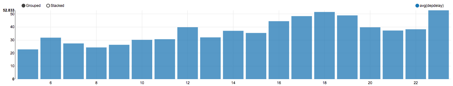
What are the four most frequent flight routes in the data set? or What is the count of flights for all possible flight routes, sorted? (Note: we will use the DataFrame returned later)
val flightroutecount=graph.edges
 .groupBy("src", "dst")
 .count().orderBy(desc("count")).show(4)

--- result: ---
+---+---+-----+
|src|dst|count|
+---+---+-----+
|LGA|ORD| 4442|
|ORD|LGA| 4426|
|LAX|SFO| 4406|
|SFO|LAX| 4354|
+---+---+-----+
result in a bar chart:

Vertex Degrees
The degree of a vertex is the number of edges that touch the vertex. GraphFrames provides vertex inDegree, outDegree, and degree operations, which determine the number of incoming edges, outgoing edges, and total edges. Using GraphFrames the degree operation we can answer the following question.
Which airports have the most incoming and outgoing flights?
graph.degrees.orderBy(desc("degree")).show(3)

--- result: ---
+---+------+
| id|degree|
+---+------+
|ATL| 60382|
|ORD| 64386|
|LAX| 53733|
+---+------+
result in a bar chart:

PageRank
Another GraphFrames query is PageRank, which is based on the Google PageRank algorithm.
PageRank measures the importance of each vertex in a graph, by determining which vertices have the most edges with other vertices. In our example, we can use PageRank to determine which airports are the most important, by measuring which airports have the most connections to other airports with lots of connections. We have to specify the probability tolerance, which is the measure of convergence. Note that the results are similar to the degrees operation, but the algorithm is different.
What are the most important airports, according to PageRank?
// use pageRank
val ranks = graph.pageRank.resetProbability(0.15).maxIter(10).run()

ranks.vertices.orderBy($"pagerank".desc).show()

--- result: ---
+-------------+-------+-----+---+------------------+
|         City|Country|State| id|          pagerank|
+-------------+-------+-----+---+------------------+
|      Chicago|    USA|   IL|ORD| 1.421132695625478|
|      Atlanta|    USA|   GA|ATL|1.3389970164746383|
|  Los Angeles|    USA|   CA|LAX|1.2010647369509115|
|       Dallas|    USA|   TX|DFW|1.1270726146978445|
|       Denver|    USA|   CO|DEN|1.0590628954667447|
|San Francisco|    USA|   CA|SFO| 1.024613545715222|
|     New York|    USA|   NY|LGA|0.9449041443648624|
|       Boston|    USA|   MA|BOS|0.8774889102400271|
|       Newark|    USA|   NJ|EWR|0.8731704325953235|
|        Miami|    USA|   FL|MIA|0.8507611366339813|
|      Houston|    USA|   TX|IAH|0.8350494969577277|
|    Charlotte|    USA|   NC|CLT|0.8049025258215664|
|      Seattle|    USA|   WA|SEA|0.6417798484556717|
+-------------+-------+-----+---+------------------+
Message Passing via AggregateMessages
Many important graph algorithms are iterative algorithms, since properties of vertices depend on properties of their neighbors, which depend on properties of their neighbors. Pregel is an iterative graph processing model, developed at Google, which uses a sequence of iterations of messages passing between vertices in a graph. GraphFrames provides aggregateMessages, which implements an aggregation message-passing API, based on the Pregel model. GraphFrames aggregateMessages sends messages between vertices and aggregates message values from the neighboring edges and vertices of each vertex.

The code below shows how to use aggregateMessages to compute the average flight delay by the originating airport. The flight delay for each flight is sent to the src vertex, then the average is calculated at the vertices.
import org.graphframes.lib.AggregateMessages

val AM = AggregateMessages
val msgToSrc = AM.edge("depdelay")
val agg = { graph.aggregateMessages
  .sendToSrc(msgToSrc)
  .agg(avg(AM.msg).as("avgdelay"))
  .orderBy(desc("avgdelay"))
  .limit(5) }
agg.show()

--- result: ---
+---+------------------+
| id|          avgdelay|
+---+------------------+
|EWR|17.818079459546404|
|MIA|17.768691978431264|
|ORD|  16.5199551010227|
|ATL|15.330084535057185|
|DFW|15.061909338459074|
+---+------------------+
Motif Find for Graph Pattern Queries
Motif finding searches for structural patterns in a graph. In this example, we want to find flights with no direct connection. First, we create a subgraph from the flightroutecount DataFrame that we created earlier, which gives us a subgraph with all the possible flight routes. Then, we do a find on the pattern shown here to search for flights from a to b and b to c, that do not have a flight from a to c. Finally, we use a DataFrame filter to remove duplicates. This shows how Graph queries can be easily combined with DataFrame operations like filter.
What are the flight routes with no direct connection?

val subGraph = GraphFrame(graph.vertices, flightroutecount)
val res = subGraph
 .find("(a)-[]->(b); (b)-[]->(c); !(a)-[]->(c)")
 .filter("c.id !=a.id”)

Shortest Path Graph Algorithm
Shortest path computes the shortest paths from each vertex to the given sequence of landmark vertices. Here, we search for the shortest path from each airport to LGA. The results show that there are no direct flights from LAX, SFO, SEA, and EWR to LGA (the distances greater than 1).
val results = graph.shortestPaths.landmarks(Seq("LGA")).run()
+---+----------+
| id| distances|
+---+----------+
|IAH|[LGA -> 1]|
|CLT|[LGA -> 1]|
|LAX|[LGA -> 2]|
|DEN|[LGA -> 1]|
|DFW|[LGA -> 1]|
|SFO|[LGA -> 2]|
|LGA|[LGA -> 0]|
|ORD|[LGA -> 1]|
|MIA|[LGA -> 1]|
|SEA|[LGA -> 2]|
|ATL|[LGA -> 1]|
|BOS|[LGA -> 1]|
|EWR|[LGA -> 2]|
+---+----------+
Breadth First Search Graph Algorithm
Breadth-first search (BFS) finds the shortest path from beginning vertices to end vertices. The beginning and end vertices are specified as DataFrame expressions, maxPathLength specifies the limit on the length of paths. Here we see that there are no Direct flights between LAX and LGA.
val paths = graph.bfs.fromExpr("id = 'LAX'")
 .toExpr("id = 'LGA'")
 .maxPathLength(1).run()

paths.show()

+----+-------+-----+---+
|City|Country|State| id|
+----+-------+-----+---+
+----+-------+-----+---+
Here we set the maxPathLength to 2. The results show some flights connecting through IAH for flights from LAX to LGA.
val paths = graph.bfs.fromExpr("id = 'LAX'")
 .toExpr("id = 'LGA'")
 .maxPathLength(2).run().limit(4)
paths.show()

You can combine motif searching with DataFrames operations. Here we want to find connecting flights between LAX and LGA using a Motif find query. We use a Motif query to search for the pattern of a flying to b, connecting through c, then we use a DataFrame filter on the the results for A=LAX and C=LGA. The results show some flights connecting through IAH for flights from LAX to LGA.
graph.find("(a)-[ab]->(b); (b)-[bc]->(c)")
.filter("a.id = 'LAX'")
.filter("c.id = 'LGA'").limit(4)

Combining a Motif find with DataFrame operations, we can narrow these results down further, for example flights with the arrival flight time before the departure flight time, and/or with a specific carrier.
Summary
GraphFrames provides a scalable and easy way to query and process large graph datasets, which can be used to solve many types of analysis problems. In this chapter, we gave an overview of the GraphFrames graph processing APIs. We encourage you to try out GraphFrames in more depth on some of your own projects.
All of the components of the use case we just discussed can run on the same cluster with the MapR Data Platform.

Code
- You can download the code and data to run these examples from here: https://github.com/mapr-demos/mapr-spark2-ebook
Related
3 ways a data fabric enables a data-first approach
Mar 15, 2022A Functional Approach to Logging in Apache Spark
Feb 5, 2021
Getting Started with DataTaps in Kubernetes Pods
Jul 6, 2021